Contents

1. FlowL
   1. What is “FlowL” ?
   2. Scalar / Vector Field of Magnetic Potential and Point Charges
   3. Components in FlowL
2. Using FlowL with Attractor Points
   1. 2D Gravity Field | example
   2. 2D Gravity Field + Vortex | example
   3. 3D Gravity Field | example

---

FlowL

What is “FlowL” ?

As the website for plug-ins / add-ons of Rhinoceros / Grasshopper, which name is Food4Rhino, says;

flowL is a plug-in to visualize a vector field, generated trough positive and negative point charges.
 The path lines are calculated with the "Runge-Kutta 4th Order Method" short "RK4", developed by the German mathematicians C. Runge and M.W. Kutta. around 1900.

Scalar / Vector Field of Magnetic Potential and Point Charges

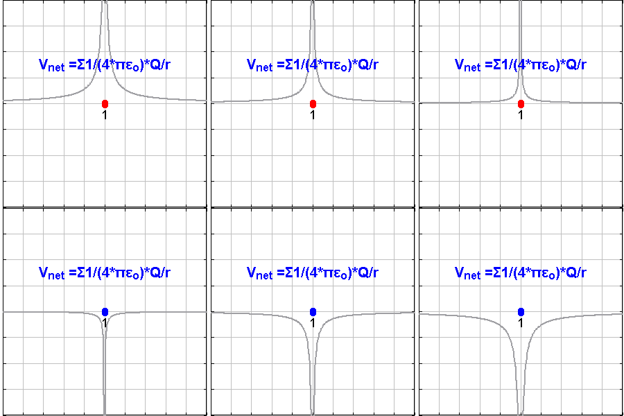
Scalar field and vector field are concepts to understand spaces filled with potential energies by looking into a matrix of points in the space with values on them. Temperature distribution and magnetic field are kinds of them.

In electric fields, point charges are the origin points of the vector / scalar field. The points with + value attract electrons, and the points with – value repulse them.

Components in FlowL

• Equi2D :    Generates isolines from sample points with the scalar field by point charges and values in 2D
• StreamLines2D :    Generates stream lines of vector field by point charges and values from sample points in 2D
• StreamLines2DVortex :    Generates stream lines of vector field by point charges and value including vortex value from sample points in 2D
• StreamLines3D :   Generates stream lines of vector field by point charges and values from sample points in 3D

Using FlowL with Attractor Points

2D Gravity Field

2D Gravity Field + Vortex

3D Gravity Field